Logistic population growth The term logistic was first invented in the nineteenth century to describe population growth curves. R intrinsic rate of natural increase.
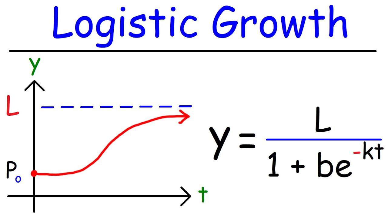
Logistic Growth Function And Differential Equations Youtube
Multiple Choice ook A population that is increasing in size but never reaches its carrying capacity.

. When studying population functions different assumptionssuch as exponential growth logistic growth or threshold populationlead to different rates of growth. A differential equation that describes logistic growth for some animal population is given by the formula. The idea is pretty simple.
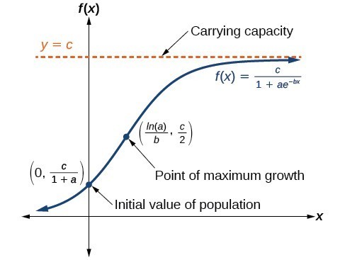
This equation was first introduced by the Belgian mathematician Pierre Verhulst to study population growth. Pt P 0 e rt where P 0 is the population at time t 0. What does the logistic growth equation describe.
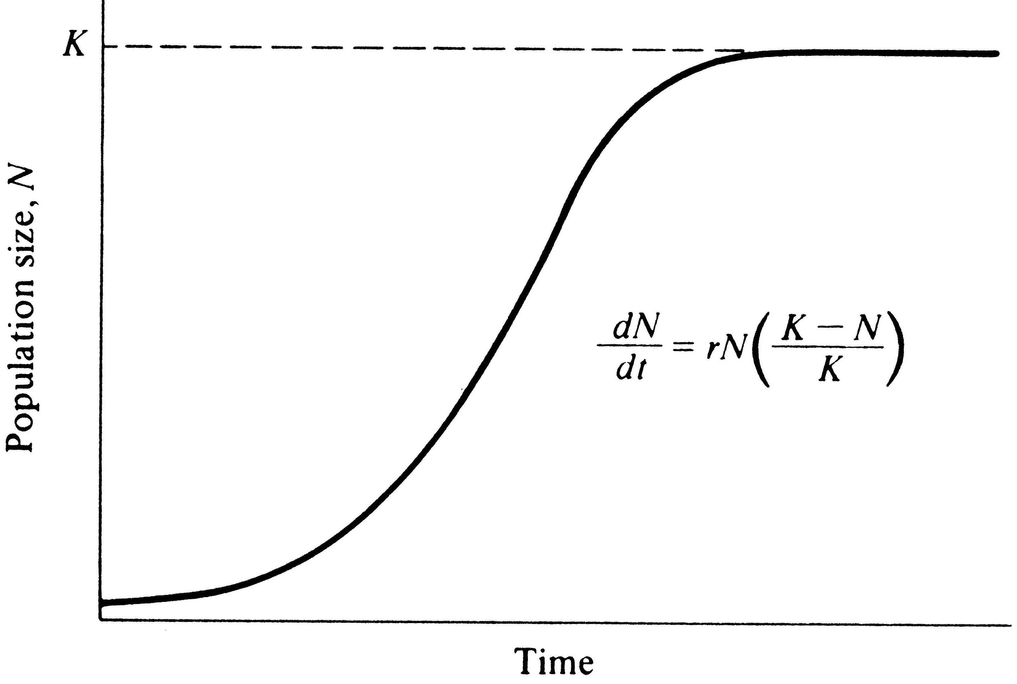
The equilibrium at P N is called the carrying capacity of the population for it represents the stable population that can be sustained by the environment. DN dt rN KN K where N population density at time t. In short unconstrained natural growth is exponential growth.
Up to 10 cash back The classical logistic equation was introduced by Verhulst as an ordinary differential equation ODE to describe population growth in a limited environmentHutchinson noted that the classical logistic equation is not appropriate when there is a lag in some of the population growth processes so he formulated a model as a delay. Let the logistic differential equation be dPdt 0004 P50-P Find. Any natural growth process consists in filling a given niche since its beginning until saturation considering that any niche to be filled exhibits a given carrying capacity.
Like the logistic growth equation it increases monotonically with both upper and lower asymptotes. We derive an alternative expression for a delayed logistic equation in which the rate of change in the population involves a growth rate that depends on the population density during an earlier time period. It is known as the Logistic Model of Population Growth and it is.
K carrying capacity. Population growth is limited so cant ever exceed some. A typical application of the logistic equation is a common model of population growth originally due to Pierre-François Verhulst in 1838 where the rate of reproduction is proportional to both the existing population and the amount.
We now solve the logistic equation 89. P t represents the population of this organism as a function of time t and the constant P 0 represents the initial population population of the organism at time t 0. This value is a limiting value on the population for any given environment.
The equilibrium solutions are P 0 and 1 P N 0 which shows that P N. Rences A population that crashes after very rapid nearly exponential growth. It is given by the following equation.
Verify that this is the solution to this logistic growth model and satisfies the initial condition. Check out the differential calculus topic for more about the notation. - 01p 1000 dp dt If the initial population is p 0 100 then the solution to this logistic growth model satisfies.
Substituting this Figure for the f N which is the function. This corresponds to a rate of increase r ln 23 02311. Also there is an initial condition that P 0 P_0.
Population ecologists usually use the symbol K for the carrying capacity so the intrinsic rate would be multiplied by K - N K. The logistic differential equation incorporates the concept of a carrying capacity. I also need to find the limit of P t as t approaches infinity.
DPdt rP where P is the population as a function of time t and r is the proportionality constant. Logistic Curve and Equation The logistic or sigmoid curve describes the natural growth process of any system. The logistic differential equation can be solved for any.
1 The carrying capacity is a constant. 2 population growth is not affected by the age distribution. Then the logistic differential equation is d P d t r P 1 P K 48 Media See this website for more information on the logistic equation.
In our formulation the delay in the growth term is consistent with the rate of instantaneous decline in the population given by the model. The logistic equation or Verhulst equation which was mentioned in Sections 11 see Exercise 61 and 25 is the equation 31 yt r aytyt where r and a are constants subject to the condition y 0 y0. Why is it called logistic growth.
The equation dP dt P 00250002P d P d t P 0025 0002 P is an example of the logistic equation and is the second model for population growth that we will consider. 3 birth and death rates change linearly with population size it is assumed that birth rates and. I need to calculate P t which will predict the population at any time.
An examination of the assumptions of the logistic equation explains why many populations display non-logistic growth patterns. The growth coefficient k The carrying capacity M The value of the population P when the rate of population growth star. A population that is declining in size and with further time may become extinct.
A population that grows steadily when the. We know that all solutions of this natural-growth equation have the form. The logistic growth causes relatively constant growth rate in the population.
The general form of the logistic equation is Pt fracKP_0ertKP_0ert-1. We have reason to believe that it will be more realistic since the per capita growth rate. The logistic equation The logistic equation is dP dt kPN P.
1P dPdt B - KP where B equals the birth rate and K equals the death rate. In this equation is the growth rate of the population in a given instant is population size is time and is the per capita rate of increase that is how quickly the population grows per individual already in the population. Population growth curve a when responses have not limited the growth the plot is exponential b when responses are limiting the growth the.
In this way the growth of a population human beings or any animal species the diffusion of epidemic or. If reproduction takes place more or less continuously then this growth rate is represented by. This assumes -- with plentiful food supply and no predation -- that the population grows exponentially which is reasonable at least in the short term The KDFWR also reports deer densities for 32 counties in Kentucky the average of which is approximately 27 deer per square mile.
Assumptions of the logistic equation. An exponential growth is an increasing growth rate in which the individuals in a population reproduce at a constant rate due to a great number of resources.
9 Population Growth And Regulation
Population Growth And Regulation
Use Logistic Growth Models College Algebra


0 Comments